Background

I did a lot of work on this project before making this site. The whole project started as a hobby and then I expanded it for a final project in a class and it's now back to a hobby with the intent of eventual publication. But what exactly is it? The goal is to recreate the synaptic weights of a neural network using indirect measurements of neural activity. Essentially, I wanted to recreate a brain from a brain scan. I never saw anything quite like this and thought I could at least try on a small scale. And I did start small. Real neurons have terribly complex time varying behavior and a nearly endless number of parameters you could tweak depending on how deep into the biophysics you really wanted to get. Similarly, there are a ton of different scanning methods available for imaging neurons all with various levels of complexity to simulate. I went with what are arguably the simplest models in each of these two areas, simple feed forward neural networks and MEG data. My question going in was this: “Is it possible to recreate the weights of a neural network with only data from the magnetic field surrounding it and the inputs to said neural network?” The answer turns out to be “yes”. By the end of this, you will hopefully understand exactly how I probed and recreated the hidden variable of a neural network and will be able to parse my code I used to do it.

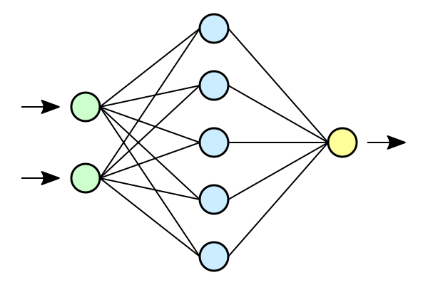
So here’s some basic background on the approach. I presume if you’re reading this, you’re familiar with machine learning. My first task was to create and train a neural network. I actually coded all that from scratch both as a learning exercise, I have no formal experience with machine learning, and to make sure I had access to all the weights with relative ease. I made a single layer neural network and used an evolutionary algorithm to train it on the iris dataset. It had 4 inputs, 10 hidden nodes, and 3 outputs. My model looks quite similar to this just with a different number of nodes.

Usually, this is just a useful abstraction to visually depict the underlying math. In this project however, the network was thought of as having this actual physical extent. Each neuron has a value associated with it. Each synapse has an associated weight. I treated each value as a voltage and each weight as a conductance. From here, I used Ohm’s law to find the current flowing in each of the synapses. (As a brief aside, in the actual code I ignored the voltage of the postsynaptic neuron as this is already non-physical. This is a useful simplifying assumption that actually has some relevance to the biological model I am working on now.) These currents in turn generate a magnetic field. I made the assumption that all current is constant and didn’t consider any propagation time through the network or the like. I probed the magnetic field at points on a grid spanning the edges of the network. It is actually pretty computationally intensive to calculate the magnetic field of these networks. I used the Biot–Savart law which required me to numerically calculate an integral. Fortunately, there is a work around that turns this into a simple matrix multiplication. Since my model doesn’t have current as a function of position, the current could be factored out of the integral. Then, I could calculate the contribution from each synapse to each sensor for a unit current. Then when it came time to calculate the sensor values for any particular state, I saved the currents for each synapse to a vector and matrix multiplied to get the desired senor values. The goal was now to use this data to recreate the underlying synaptic weights of a network.

So, how would one go about recreating the network? My initial approaches were suboptimal to put it lightly. I mentioned I used a genetic algorithm to train the initial model. That was partly because I was too lazy to implement my own backpropagation algorithm. However, I knew that backpropagation would not be suited to the recreation as my loss function would be completely unrelated to the model’s output. But evolution is blind to what I’m trying to optimize and I thought I could just throw anything at it. How wrong I was. Evolution will give a locally optimal solution, it works with what it has. This is usually fine, there are many ways to get very good behavior and that's why it worked in the initial classification. But for this problem, it needed to be exact. If the magnetic field was close but the weights were still far off, it would get stuck in that local optimum and be miles away from what I wanted with no way to change. I needed something more structured, something to solve analytically or close to it.

It turns out the magnetic field sensor values can be written as a terribly complex system of equations. For all the weights in the first layer, their contribution was easy. Their input node value, a value known and set by the iris data set, multiplied by their weight gave the current. This current times a constant factor gave this particular synapse's contribution to the magnetic field at a certain sensor point. The weights in the next layer, connecting the hidden neurons to the output, were not as easy. The values of the hidden neurons were not know as their were determined by the weights and the activation function. So, everything had to be left in terms of the weights from the previous layer. Had I added more layers this process would have gone backwards again and again. I appreciate the verbal explanation may be less than clear. It is my hope that the following equation helps this.

I can see that this also isn't going to be self explanatory. Let's go through each variable and subscript explaining what everything means. For starters, S1 is the first sensor value. There was a grid of sensors so we need some way to tell them apart. In1 is the input value of the first node. This is set by the iris dataset. wi11 is the weight connecting the first input neuron to the first hidden neuron. Similarly, wi12 is connecting the first input neuron to the second hidden neuron. ci111 is the conversion factor from current at in the synapse connecting the first input neuron and first hidden neuron to magnetic field strength at the location of the first sensor. So the indices in order are sensor index, input index, hidden index. The i's and h's after w's and c's represent input and hidden respectively. The arctangent function is the activation function I used in this project. It has the advantage of being differentiable with is useful later. The argument in the arctangent function will yield the value of the hidden nodes. In total, I had 70 synapses which means 70 independent variables. I ended up using an 8x8 sensor array giving 64 sensors total. The keen eyed among you will realize with 64 measurements and 70 variables, the system is under constrained and thus, unsolvable. Of course, I could just take measurements with different input values and get 64 new measurements which would over constrain the system. As it turns out, the method I used to solve for these weights required the system to be highly over constrained to avoid local minima. The next section will be devoted to describing how I solved a system of hundreds of non linear equations.

Have you ever wondered what actually happens when a program approximates a function of best fit to measured data? It isn't something I ever thought about before this project. One method is called the Gauss-Newton algorithm. The method actually isn't terribly complex, especially for simple functions like low order polynomials. Before explaining the Gauss-Newton algorithm, I think I should explain Newton's method of finding roots. Imagine you have a polynomial equation and you want to find the points where . Not exactly a challenge to solve algebraically but it will serve as a useful example. Pick a random point on this curve, let's say . Now taking the derivative at this point we will get . We can apply the equation to get an updated value closer to the solution. In this case, .

The Gauss-Newton method generalizes this to systems of equations. The mathematical rigor is likely beyond my ability to explain. With multiple variables, the full derivatives must be substituted for partial derivatives. Instead of single variables, the variables are represented as a vector and the derivatives are put into a matrix which acts upon the function of this vector. The form is very similar and is shown here: . The tricky part is finding the matrix A. I think a suitable explanation would double the length of this article. A is the pseudo-inverse of the opposite of the Jacobian of the system. If you know what that means that's fantastic. If you don't it really isn't relevant to the overall idea. That overall idea being, by taking derivatives of the system and taking multiple iterations, we can approach the solution to an arbitrary system of equations, including the huge set of equations generated by the magnetic field data.

The downsides of this method are that its very computationally intensive and that it can also get trapped in local minima. When I was running the first tests of this method, I was using a 4x4 sensor array, so 16 total. I thought that would be more then enough to constrain the system provided I had 5 or more distinct measurements giving at least 80 equations and only 70 weights to recreate. What happened here was getting caught in local minima. I think the problem could be solved with this method and 16 sensors but I have some caveats. First, it could just run multiple times, eventually the random initial guesses could possibly result in movement only toward the global optimum, not likely but possible. Second, I could have tons of measurements. If I had 50 or more distinct inputs, the problem would likely be solved. However, this goes back to the computationally intensive part. This algorithm requires taking the matrix inverse at each step. Such a calculation was taking upwards of 20 minutes on my machine if I remember correctly. It would likely have taken days which I wasn't willing or able to wait for when I was finishing this project up during my finals week. Even with 8x8 sensors, it wasn't as easy as just two distinct measurements. In my code I used 5 for a total of 8x8x5 or 320 measurements. Even with this, convergence was slow and getting stuck in local minima was possible. Crucially though, it did solve and that was all the proof of concept I needed.

And what now? Now I'm working on making biologically inspired neural networks and doing the same kind of recreation. Just the basic neuron model deserves its own post and this is already too long. I will write that up when I have the chance. After that I can really dig into the progress and challenges I am facing with the actual recreation as the method described above is not viable. If you're interested in this project or what is to come, here is the github link to see the code. It's messy but it works.